O&G Unit Converter V2.5

Pipe Volume Calculator

INNER DIAMETER

LENGTH

CALCULATED VOLUME

0.000

Z-Factor Estimator (Papay)

SPECIFIC GRAVITY (Air = 1.0)

PRESSURE

TEMP

ESTIMATED COMPRESSIBILITY

Z-Factor

0.0000

Petroleum Gravity (°API ↔ SG ↔ Density)

API GRAVITY (°API, 60/60 °F)

SPECIFIC GRAVITY (water = 1)

DENSITY (at 60 °F)

°API = 141.5 / SG − 131.5 · density = SG × 999.016 kg/m³ (water at 60 °F, ASTM D1250 basis).

Viscosity (Dynamic ↔ Kinematic)

DYNAMIC VISCOSITY (μ)

KINEMATIC VISCOSITY (ν)

DENSITY (ρ) — required to bridge

ν = μ / ρ · 1 cSt = 1 mm²/s · 1 cP = 1 mPa·s. Water at 20 °C ≈ 1 cP ≈ 1 cSt.

Mass ↔ Volumetric Flow (by density)

MASS FLOW

VOLUMETRIC FLOW

DENSITY (ρ) — at flowing conditions

Q_vol = ṁ / ρ. For gases, use the density at the stated T & P (or the compositional ρ_std from the Advanced tab).

Gas Heating Value (Compositional) & Flow

Input Mode:

1. GAS COMPOSITION

*C6+ evaluated as nC6.

CH₄

C₂H₆

C₃H₈

iC₄

nC₄

iC₅

nC₅

nC₆+

C₂H₄

C₃H₆

H₂

CO₂

N₂

O₂

Total Input Fraction 100.00%

2. Conditions & Operating State

Temperature

Pressure

LNG Liquid Temp (For Liquid Density)

CALCULATED OPPOSITE FRACTIONS

3. Physical & Combustion Properties

HV:

Heating Value (HHV)

0.00

Mol. Weight (MW)

0.000 g/mol

Specific Gravity (Air = 1)

0.000

Wobbe Index (WI) HHV-based

0.00

Max Comb. Potential (MCP)

0.0

Liquid Density (LNG approx)

0.00

4. Mass & Volumetric Flow Conversions

Given Mass Flow

Calculated Output (A)

0.00

Given Volumetric Flow

Calculated Output (B)

0.000

Pipe Delta Pressure Calculator (Darcy-Weisbach)

1. SYSTEM & PIPE PARAMETERS

SCALING FACTOR

SYSTEM PRESSURE

PIPE ID

ROUGHNESS

PIPE LENGTH

ELEVATION CHANGE

EROSION C-FACTOR (API RP 14E)

2A. VAPOR PHASE

MASS FLOW

DENSITY

DYNAMIC VISCOSITY

2B. LIQUID PHASE

MASS FLOW

DENSITY

DYNAMIC VISCOSITY

3. HYDRAULIC OUTPUTS

Awaiting Calc...

TOTAL dP

0.00

dP / LENGTH

0.00

VELOCITY

0.00

Reynolds No.

—

Darcy Friction f

—

Colebrook-White

Erosional V_e

— m/s

v / V_e = —

Erosion Check —

Flow Regime

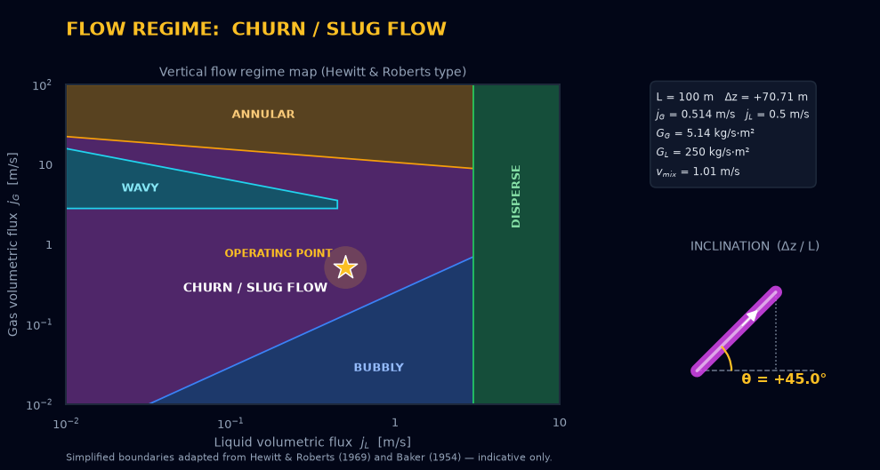
Awaiting Visualization...

Visualizes the two-phase flow pattern from the inputs of the Pipe Delta Pressure Calculator above. Inclination θ = asin(Δz / L) is taken from PIPE LENGTH and ELEVATION CHANGE. |θ| ≥ 30° uses the vertical-flow map (Hewitt & Roberts type); |θ| < 30° uses the horizontal-flow map (Baker type). The map is rendered server-side with Python seaborn. Boundaries are simplified — indicative only.

PRV Sizing Calculator (API 520 Part I)

Units:

Mode:

Gas / Vapor Inputs (§5.6)

MASS FLOW W

lb/h

MOL. WEIGHT M

g/mol

HEAT RATIO k (Cp/Cv)

—

RELIEVING TEMP T

°R

COMPRESSIBILITY Z

—

RELIEVING PRESS P1

psia

BACKPRESSURE P2

psia

Kd [0.975 PRV; 0.62 rupture disk]

Kb [1.0 conventional/pilot]

Kc [1.0 no disk; 0.9 with disk]

P1 = Set Pressure × (1 + OP%) + P_atm. Critical vs. Subcritical auto-detected: Pcf = P1 × (2/(k+1))^(k/(k−1)).

Sizing Results

Awaiting Calc...

REQUIRED AREA A

— in²

API 526 ORIFICE

—

ORIFICE AREA

—

Run calculation to see intermediate values (C, Pcf, KN, ω, η_c, G, Kv, Re…)

⚠ Preliminary sizing only per API 520 §5.6–§5.10. Final PRV selection requires independent engineering review, manufacturer-certified Kd, and compliance with applicable codes (ASME, local regulations).

How To Use — Operations Manual v2.5

A step-by-step visual guide covering every panel of the O&G Engineering Converter. Use the wireframe diagrams and annotations to master each feature.

★ New in Version 2.5

Navigation & accessibility — the active tab now scrolls into view on narrow screens, tab buttons expose proper ARIA tab semantics for screen readers, and the long How To Use / Theory pages gained jump links and a floating Top button.

Calculator ergonomics — press Enter in any ΔP or PRV input to calculate; missing required inputs show an instant hint instead of a failed server call; editing inputs after a result flags the status badge with inputs changed — recalculate.

Robustness — Export PDF falls back to an HTML download when pop-ups are blocked, and viscosity unit selections (mPa·s, mm²/s) are preserved across reloads and share links.

Documentation — the GitHub repository now ships a docs/ folder: Development Plan (history & roadmap), Detailed Specification of every module and API, and a promotion strategy. Theory §4.1 now correctly documents the Papay Z-factor method.

★ New in Version 2.4

ΔP card relabelled — the pressure-drop method is correctly named Darcy-Weisbach (it always was; the old "Fanning" label was a misnomer). Outputs now also report Reynolds number, the Darcy friction factor f, and an API RP 14E erosional-velocity check (set the C-factor in the inputs).

Flow-regime cross-link — once you visualise the flow regime, the result is echoed inside the ΔP output panel for a single-glance read.

Out-of-range warnings — the LNG density (ISO 6578, 108–120 K), gas composition (negatives / off-100% totals), and Papay Z-factor (Pr/Tr envelope) now flag extrapolated inputs instead of silently clamping.

New Basic Eng converters — Petroleum Gravity (°API ↔ SG ↔ density), Viscosity (dynamic ↔ kinematic), and Mass ↔ Volumetric flow (by density).

Export PDF report — the floating Export PDF button (bottom-right) opens a printable summary of every current calculation; use your browser's "Save as PDF".

Share & auto-restore — the Share button copies a link that reproduces all your inputs; the app also restores your last session automatically from local storage.

Note on units — in the Advanced flow section, when Temperature ≠ 0 °C or Pressure ≠ 0, outputs are in actual cubic metres (kAm³/h), not standard normal cubic metres (kNm³/h). A red banner appears whenever you leave standard conditions.

1. Application Header & Tab Navigation

The dark header bar contains all navigational tabs. Click any tab to switch context. The active tab shows an amber underline.

⚙ O&G ENG CONVERTER v2.4 • Hybrid

General Basic Eng Advanced How To Use Theory Terms of Use Privacy Report

▲ amber = active tab | grey = inactive

2. General Tab — Standard Converter Blocks

Pre-built converter cards for the most common O&G unit pairs. Each card has two input fields; editing either side auto-converts the other.

STANDARD CARD (e.g. Pressure)

INPUT →

101.325

⇅

OUTPUT →

14.696

STANDARD CARDS AVAILABLE

Nm³ ↔ scf (gas volume)

Pressure (kPa, bar, MPa, psi) — with Abs/Gauge toggle per side

Temperature (°C, °F, K)

Heating Value (MJ/Nm³ ↔ BTU/scf)

Custom Modules (user-created)

📋 Copy to Clipboard: Click the clipboard icon next to any output field to instantly copy the value for use in reports or spreadsheets.

🔵 Pressure Abs/Gauge Toggle: Each pressure side (A and B) has an independent Abs / Gauge toggle button. Set each side to Absolute or Gauge independently before entering a value. The conversion always routes through Pa absolute internally, using 101,325 Pa (1 atm) as the atmospheric reference. Example: 101,325 Pa (Abs) = 0 Pa (Gauge) = 1 atm.

3. Custom Modules — Configure & Save

Create unlimited custom unit converters using a linear multiplier (Unit1 × Factor = Unit2). Saved to browser Local Storage — persists across sessions.

CONFIGURE MODULE MODAL

QUICK LOAD TEMPLATE

MODULE IDENTIFIER

Crude Oil

UNIT 1

Metric Tons

UNIT 2

Barrels (bbl)

MULTIPLIER FACTOR

7.33

Abort Initialize

CREATED CARD EXAMPLE

Crude Oil TERMINATE

Metric Tons

1.00

⇅

Barrels (bbl)

7.33

↑ Click TERMINATE to permanently delete this module.

4. Basic Eng Tab — Various Calculators

Two engineering calculators for pipe geometry and gas compressibility. Each is independent and requires its own inputs.

PIPE VOLUME

Inner Diameter → mm or inch

Length → m, ft, mile, km

→ Volume [m³, bbl, gallon]

Z-FACTOR (Papay)

Specific Gravity, T, P inputs

Papay correlation method

→ Z compressibility factor

ℹ Pipe Delta Pressure Calculator is located in the Advanced tab, not here. It supports single-phase and two-phase (HEM) flow, with server-side computation via Colebrook-White iterative friction factor (Python / Vercel API) — see Section 9 for the full walkthrough. Since v2.3, a Flow Regime visualizer card sits directly beneath it (see Section 10 below).

5. Advanced Tab (Section 1) — Gas Composition Input

Enter the percentage of each component. The total must sum to 100%. Choose between Volumetric Fraction (%) or Mole Fraction (%) input mode.

1. GAS COMPOSITION INPUT

Vol% Mol%

CH₄ (Methane)

89.00 %

C₂H₆ (Ethane)

7.00 %

C₃H₈ (Propane)

2.50 %

N₂ (Nitrogen)

0.30 %

Total Input Fraction 100.00%

⚠ Total shown in red if ≠ 100%. All calculations use normalized fractions regardless.

6. Advanced Tab (Section 2) — Operating Conditions

Override standard conditions (0°C, 0 MPaG) to compute actual volumetric flows at operating pressure and temperature. LNG liquid temp is only used for liquid density calculation.

2. CONDITIONS & OPERATING STATE

Temperature

0°C

Standard ✓

Pressure (gauge)

0MPaG

Standard ✓

LNG Liquid Temp

-160°C

For density only

⚠ If T≠0°C or P≠0, flow is in actual m³ (Am³), not standard Nm³. Column labels change to kAm³/h.

7. Advanced Tab (Section 3) — Physical & Combustion Properties

All outputs computed per JIS K 2301 (2011) using Z-corrected mole fractions. Use the HHV / LHV toggle inside the Section 3 header row to switch between Higher (総発熱量) and Lower (真発熱量) Heating Value modes. Results update automatically. Note: Wobbe Index always uses HHV per JIS K 2301 §7 regardless of mode.

3. PHYSICAL & COMBUSTION PROPERTIES

Heating Value (HHV)

44.59

MJ/Nm³

Mol. Weight (MW)

18.305

g/mol

Specific Gravity

0.634

Air = 1

Wobbe Index (HHV)

56.00

MJ/Nm³

Liquid Density

~466

kg/m³ @-162°C

HHV/LHV Toggle: In LHV mode, Heating Value shows 真発熱量 from JIS K 2301 Table 30. LHV (ref. example) = 40.25 MJ/Nm³. WI, SG, MW and density outputs are unaffected by this toggle.

Calculated Molar Fractions (Vol% mode input → Mol% displayed)

CH4: 88.87 C2H6: 7.04 C3H8: 2.54 N2: 0.30

8. Advanced Tab (Section 4) — Mass & Volumetric Flow Conversions

Two independent sub-panels: (A) Given Mass → Calculated Output and (B) Given Volume → Calculated Output. Each output panel has a toggle button (VOL/MOL for panel A; MASS/MOL for panel B) to switch between the standard flow output and Molar Flow. Available units: Mass: kg/s, kg/h, ton/h, ton/d, lb/h, lb/d. Molar: kmol/h or mol/s.

🔵 VOL/MOL and MASS/MOL Toggles: When MOL mode is selected, the output panel displays Molar Flow calculated as ṁ[kg/h] ÷ MW[g/mol] = n_dot[kmol/h]. Select kmol/h or mol/s from the unit dropdown. These molar flow values are useful for combustion air calculations, pipe sizing, and heat exchanger duties.

A. MASS → VOLUME

Given Mass Flow

100

↓ ÷ ρ_std

Calculated Volumetric Flow

122.06

B. VOLUME → MASS

Given Volumetric Flow

100

↓ × ρ_std

Calculated Mass Flow

81.930

ℹ Reference values (CH₄=89%, C₂=7%, C₃=2.5%, iC₄=0.7%, nC₄=0.5%, N₂=0.3%):
100 ton/h → 122.056 kNm³/h | 100 kNm³/h → 81.930 ton/h (matches JIS K 2301 / Excel exactly)

9. Advanced Tab — Pipe Delta Pressure Calculator (Darcy-Weisbach)

Computes the pressure drop along a pipe for single-phase (vapor or liquid) and two-phase flow; the two-phase case uses the Homogeneous Equilibrium Model (HEM). The iterative Colebrook–White friction factor and the full Darcy–Weisbach solution run server-side (Python / Vercel API). Enter the pipe geometry and per-phase properties, then click CALCULATE PRESSURE DROP. The phase regime — Single-Phase Vapor, Single-Phase Liquid, or Two-Phase (HEM) — is auto-detected from which mass flows are non-zero and shown as a badge.

INPUTS — 1. SYSTEM & PIPE

Scaling factor — multiplies both phase mass flows

System pressure · Pipe ID · Roughness ε (default 0.045 mm, commercial steel)

Pipe length L · Elevation change Δz (sets static head ρ·g·Δz)

Erosion C-factor — API RP 14E: 100 continuous, 125 intermittent

INPUTS — 2A / 2B. PHASE PROPERTIES

Vapor & Liquid each: mass flow · density · dynamic viscosity

Leave a phase’s mass flow at 0 to model single-phase flow

3. HYDRAULIC OUTPUTS

Total ΔP [bar / psi / Pa / kPa / MPa] = friction + static head

ΔP / length · mixture Velocity

Reynolds number + regime [Laminar / Transitional / Turbulent]

Darcy friction factor f (Colebrook–White)

Erosional velocity V_e = C/√ρ, ratio v/V_e, with badge WITHIN / NEAR / EXCEEDS

→ A visualised two-phase regime is echoed here (see Section 10)

ℹ Default inputs (ID = 4 in, L = 100 m, Δz = 70.711 m, vapor 150 kg/h @ 10 kg/m³ / 0.012 cP, liquid 7,300 kg/h @ 500 kg/m³ / 0.12 cP) give ΔP ≈ 176.9 kPa (≈ 2.3 kPa friction + 174.6 kPa static head), v ≈ 1.01 m/s, Re ≈ 2.2×10⁵ (turbulent), f ≈ 0.018, V_e ≈ 7.72 m/s at C = 100 → v/V_e ≈ 0.13 (WITHIN LIMIT). The two-phase HEM neglects slip and the acceleration term — treat it as a first-pass estimate.

10. Advanced Tab — Flow Regime Visualizer

Located directly beneath the Pipe Delta Pressure Calculator and driven by the same inputs. Click VISUALIZE FLOW REGIME to classify the two-phase flow pattern on a regime map rendered server-side (Python seaborn / Vercel API), followed by a conceptual 3D animation (Three.js) of how the flow would appear inside the pipe — phase distribution, relative speed and inclination.

MAP SELECTION

θ = asin(Δz / L) — from PIPE LENGTH & ELEVATION CHANGE

|θ| ≥ 30° → Vertical map (Hewitt & Roberts type) — axes j_G vs j_L [m/s]

|θ| < 30° → Horizontal map (Baker type) — axes G_G vs G_L [kg/s·m²]

→ Regimes: Bubbly / Churn-Slug / Wavy / Stratified / Annular / Disperse

ERROR CONDITIONS (red message instead of map)

|Elevation change| > pipe length (geometrically impossible)

Single-phase or zero flow (map needs both phases)

Non-positive pipe ID or length

Vapor density ≥ liquid density (impossible phase properties)

ℹ Default inputs (ID = 4 in, L = 100 m, Δz = 70.711 m, vapor 150 kg/h @ 10 kg/m³, liquid 7,300 kg/h @ 500 kg/m³) produce Churn / Slug Flow at θ = +45.0° (j_G ≈ 0.51 m/s, j_L ≈ 0.50 m/s, vertical map). Map boundaries are simplified — indicative only, not for design.

Example output for the default inputs — the seaborn regime map (top) and a frame of the Three.js 3D animation (bottom):

Example flow regime map: Churn / Slug Flow at +45° on the vertical (Hewitt & Roberts type) map, with operating point and inclination schematic. — Flow regime map (Python seaborn, server-side) — Churn / Slug Flow, θ = +45.0°, vertical map.

Example 3D flow animation: liquid slugs and bullet-nosed Taylor gas bubbles travelling up a pipe inclined at 45 degrees. — 3D flow animation (Three.js) — slug flow in a 45° inclined pipe. Live in-app; conceptual, not a CFD result.

11. Safety Tab — PRV Sizing (API 520 Part I)

Sizes Pressure Relief Valves (PRVs) per API Standard 520 Part I §5.6–§5.10 and Annex C. Select the sizing mode and unit system, enter process inputs, then click CALCULATE ORIFICE SIZE to obtain the required effective discharge area and the recommended API 526 orifice letter designation (D–T).

SIZING MODES

§5.6Gas / Vapor — Critical (Eq. 2/5) or Subcritical (Eq. 12/15); flow regime auto-detected vs. Pcf

§5.7Steam — Napier equation (Eq. 21/22) with KN and KSH corrections

§5.8Liquid, Certified PRV — iterative viscosity correction Kv (Eq. 28/29)

§5.9Liquid, Non-Certified — Kp overpressure correction (Eq. 38/39)

§5.10Two-Phase — Omega Method, Annex C.2.2 (Eq. C.12–C.21)

KEY OUTPUTS

Required effective area A [in² or mm²]

API 526 orifice letter [D through T]

API 526 orifice standard area [next size ≥ A]

Flow regime [Critical / Subcritical]

Intermediate values [C, Pcf, KN, ω, η_c, G, Kv, Re]

⚠ Engineering Disclaimer: Results are for preliminary sizing only. Final PRV selection requires independent review by a qualified engineer, confirmation of rated Kd with the valve manufacturer, and compliance with applicable codes.

12. Report Tab — Bug Reports & Feature Requests

Select report type, enter your name and description, then click GENERATE EMAIL TO DEVELOPER. Your default email client will open with a pre-filled message addressed to the developer.

Theory & Specifications Manual

Complete technical reference for all formulas, standards, coefficients and algorithmic logic implemented in v2.5. Primary reference: JIS K 2301:2011 and ISO 6578:1991.

Part I — Gas Compositional Analysis (JIS K 2301:2011)

1.1 Component Physical Constants (JIS K 2301 Table)

All component constants are sourced directly from JIS K 2301:2011. The compressibility factor Zᵢ and √bᵢ are key to Z-correction; Hᵢ is gross calorific value at 0°C, 101.325 kPa.

Component	MW (g/mol)	Zᵢ	HHV (MJ/Nm³)	LHV (MJ/Nm³)	√bᵢ	Sᵢ (Air=1)	Flame Spd (cm/s)
CH₄	16.043	0.9976	39.84	35.818	0.049	0.554	35.9
C₂H₆	30.07	0.9900	69.79	63.76	0.100	1.039	41
C₃H₈	44.097	0.9789	99.22	91.18	0.1453	1.523	41
iC₄H₁₀	58.123	0.9580	128.23	118.18	0.2049	2.008	38
nC₄H₁₀	58.123	0.9572	128.66	118.61	0.2069	2.008	38
N₂	28.0135	0.9995	0	0	0.0224	0.968	—
CO₂	44.01	0.9933	0	0	0.0819	1.520	—
H₂	2.016	1.0006	12.788	10.777	0	0.0696	282

1.2 Volumetric → Mole Fraction Conversion (JIS K 2301 §7)

Step 1

Cm_i = Cvᵢ / Zᵢ (un-normalized mol proportional)

Cvᵢ = volumetric fraction of component i; Zᵢ = pure-component compressibility at standard conditions

Step 2

Cmᵢ = ROUND( Cm_i / Σ Cm , 4 ) [Cm_i % — rounded to 4 d.p.]

Cmᵢ = normalized mole fraction. Rounding to 4 d.p. is mandated by the Excel reference (JIS K 2301 calculation worksheet)

Reverse

Cvᵢ (recovered) = ( Cmᵢ × Zᵢ ) / Σ(Cm × Zₖ) [Cvᵢ]

Mol% input mode: user enters Cmᵢ → displayed vol fracs follow the Cvᵢ (recovered) formula

1.3 Sample Gas Compressibility Factor (Z)

Cmᵢ × √bᵢ = ROUND( Cmᵢ × √bᵢ , 5 ) [rounded per-component to 5 d.p.]

Z = 1 − (Σ Cmᵢ × √bᵢ)²

Z_rounded = ROUND(Z, 4) [used for FLOW density calculation]

Example (CH₄=89%, C₂=7%, C₃=2.5%, iC₄=0.7%, nC₄=0.5%, N₂=0.3%):

Σ Cm√b = 0.8887×0.049 + 0.0704×0.1 + 0.0254×0.1453 + ... = 0.05693

Z = 1 − 0.05693² = 0.9968 (4 d.p.)

⚡ CRITICAL: Z_exact (before rounding) is used for HHV/SG calculations; Z_rounded (4 d.p.) is used for standard gas density ρ_std. This matches the Excel-based Calc. sheet exactly.

1.4 Gross Calorific Value / HHV

H = ROUND( Σ(Cmᵢ × Hᵢ) / Z_exact , 2 ) [MJ/Nm³]

No per-component rounding of Cmᵢ×Hᵢ before summing. Z_exact = 1−(ΣCm√b)². Final result rounded to 2 d.p. → 1.4 Gross Calorific Value / HHV.

Reference example:

Σ(Cmᵢ×Hᵢ) = 0.8887×39.84 + 0.0704×69.79 + ... = 44.444

H = 44.444 / 0.9968 = 44.587... → 44.59 MJ/Nm³

1.5 Specific Gravity & Wobbe Index

S = ROUND( Σ(Cmᵢ × Sᵢ) / Z_exact , 3 ) [Air=1]

WI = ROUND( H₂ dp / √(S₃ dp) , 2 ) [MJ/Nm³]

Sᵢ = specific gravity of pure component i relative to air. WI uses the already-rounded H (2 d.p.) and S (3 d.p.) — not the exact intermediate values. This is critical for matching Wobbe Index = 56.00.

S = 0.6321 / 0.9968 = 0.634 (3 d.p.)

WI = 44.59 / √0.634 = 55.997... → 56.00

1.6 Maximum Combustion Point (MCP)

Base MCP = ROUND( Σ(Aᵢ × fᵢ × SFᵢ) / Σ(Aᵢ × fᵢ) , 2 )

Aᵢ = vol% of combustible component i; fᵢ = combustibility factor; SFᵢ = flame speed (cm/s)

K correction (inert dilution):

denom = 100 − 4.77 × pO₂

K = (ΣAᵢ/ΣAᵢaᵢ) × [ (2.5·pCO₂ + pN₂ − 3.77·pO₂)/denom + ((pN₂−3.77·pO₂)/denom)² ]

MCP = ROUND( Base_MCP × (1 − K) , 1 )

1.7 Lower Heating Value (LHV) — 真発熱量 (JIS K 2301 Table 30)

LHV = ROUND( Σ(Cmᵢ × LHVᵢ) / Z_exact , 2 ) [MJ/Nm³]

Formula mirrors HHV (§1.4). LHVᵢ is the net calorific value of pure component i at standard conditions (0°C, 101.325 kPa, gaseous water as product) from JIS K 2301:2011 Table 30. Same Z_exact denominator and 2 d.p. rounding apply.

LHVᵢ = HHVᵢ − n_H₂O × ΔHvap(H₂O,0°C) / Vm

ΔHvap correction ≈ 2.00 MJ per Nm³ per mol H₂O (H₂: 1 mol H₂O; CH₄: 2; C₂H₆: 3; etc.)

⚠ Wobbe Index always uses HHV regardless of mode — per JIS K 2301 §7 definition.

⚠ All LHV values from JIS K 2301:2011 Table 30. ΔHvap(H₂O) implied = 2.011 MJ/Nm³ per mol H₂O at 0°C (anchored on CH₄ = 35.818 MJ/Nm³).

Reference example (same composition as §1.4):

Σ(Cmᵢ×LHVᵢ) = 0.8887×35.818 + 0.0704×63.76 + 0.0254×91.18 + ... = 40.116...

LHV = 40.116 / 0.9968 = 40.246... → 40.25 MJ/Nm³

Part II — Standard Gas Density & Flow Conversions

2.1 Standard Gas Density ρ_std

ρ_std = P·(MW/1000) / (Z_rounded·R·T_std) [kg/Nm³]

P = 101325 Pa (1 atm, standard)

MW = Σ(Cmᵢ × MWᵢ) [g/mol], where Cmᵢ is rounded to 4 d.p.

Z_rounded = ROUND(1 − (ΣCm√b)², 4) ← ROUNDED Z used here for exact Excel match

R = 8.31446262 J/(mol·K); T_std = 273.15 K (0°C)

Reference: CH₄=89%, C₂=7%, C₃=2.5%, iC₄=0.7%, nC₄=0.5%, N₂=0.3%

MW = 18.3049839 g/mol, Z_rounded = 0.9968

ρ_std = 101325 × (18.3049839/1000) / (0.9968 × 8.31446262 × 273.15) = 0.81930 kg/Nm³

2.2 Mass ↔ Volume Flow Conversion

Mass → Volume (standard):

Q_std = ṁ / ρ_std [Nm³/h]

Output units: kNm³/h (÷1000), kNm³/d (÷1000×24), mscfd

100 ton/h = 100,000 kg/h

→ 100,000 / 0.81930 / 1000 = 122.056 kNm³/h

Volume → Mass (standard):

ṁ = Q_std × ρ_std [kg/h]

Input units: kNm³/h (×1000), kNm³/d (×1000÷24), mscfd

100 kNm³/h = 100,000 m³/h (Nm³)

→ 100,000 × 0.81930 / 1000 = 81.930 ton/h

Actual Conditions (non-standard T, P):

Q_act = Q_std × (T_act/T_std) × (P_std/P_act)

Applies ideal gas temperature/pressure correction. When T≠0°C or P≠0 gauge, output units switch from kNm³/h to kAm³/h.

Part III — LNG Liquid Density (ISO 6578:1991 Klosek-McKinley)

3.1 Klosek-McKinley Method Overview

The ISO 6578 Klosek-McKinley method computes LNG liquid density by summing the molar volumes of pure-component liquids, then applying correction factors k₁ and k₂ for CH₄ and N₂ interactions.

V_mix = Σ(xᵢ · Vmᵢ(T)) − x(CH₄)·k₁(MW,T) − x(N₂)·k₂(MW,T)

ρ_LNG = MW_mix / V_mix [kg/m³]

xᵢ = mole fraction; Vmᵢ(T) = molar volume at temperature T [m³/kmol]; k₁, k₂ = correction factors from ISO 6578 Table C, interpolated by MW_mix

3.2 Molar Volume Table (ISO 6578 Table B.2) — Selected Values [m³/kmol]

Temp (K)	CH₄	C₂H₆	C₃H₈	iC₄	nC₄	N₂
108 K	0.037489	0.047513	0.062047	0.077842	0.076392	0.043571
110 K	0.037739	0.047683	0.062220	0.078040	0.076582	0.044887
111.15 K (-162°C)	0.037886	0.047776	0.062319	0.078153	0.076687	0.045660
112 K	0.037995	0.047845	0.062392	0.078236	0.076765	0.046231
114 K	0.038262	0.048014	0.062574	0.078438	0.076957	0.047602
116 K	0.038539	0.048192	0.062765	0.078648	0.077157	0.049003
120 K	0.039130	0.048576	0.063174	0.079094	0.077584	0.051906

Interpolated values computed by linear interpolation between adjacent temperature rows. Highlighted row shows the exact interpolated values at -162°C (111.15 K) from the Excel reference.

3.3 k₁, k₂ Correction Factors (ISO 6578 Table C)

MW_mix (g/mol)	k₁ (×10⁻³)	k₂ (×10⁻³)
16	−0.0086	−0.0204
17	+0.204	+0.374
18.305 (ref)	+0.465	+0.732
19	+0.580	+0.878
20	+0.776	+1.058

k₁ and k₂ are linearly interpolated by MW_mix. For the reference composition (MW=18.305): k₁≈0.465×10⁻³, k₂≈0.732×10⁻³.

Part IV — Hydraulics & Gas Laws (Advanced Tab)

4.1 Z-Factor: Papay Method (Standing-Katz Pseudo-Criticals)

Pseudo-criticals (Standing-Katz, from gas SG γ): P_pc = 756.8 − 131.0·γ − 3.6·γ² [psia] T_pc = 169.2 + 349.5·γ − 74.0·γ² [°R]

Pseudo-reduced vars: P_pr = P/P_pc T_pr = T/T_pc

Papay (1968) explicit correlation — no iteration required:

Z = 1 − 3.52·P_pr / 10^(0.9813·T_pr) + 0.274·P_pr² / 10^(0.8157·T_pr)

Validity: 0 < P_pr ≤ 15 and 1.05 ≤ T_pr ≤ 3.0 — results outside this envelope are flagged as extrapolated

4.2 Pressure Drop: Darcy-Weisbach + Colebrook-White Friction Factor

ΔP = f·(L/D)·(ρ·v²/2) + ρ·g·Δz [Pa]

Iterative Colebrook-White equation — turbulent regime (Re ≥ 2300):

1/√f = −2·log₁₀( ε/(3.7·D) + 2.51/(Re·√f) )

Laminar regime (Re < 2300): f = 64/Re

Solved iteratively to convergence (tolerance = 1×10⁻⁶, max 100 iterations)

ε = pipe absolute roughness [m]; default 0.045 mm (commercial steel)

Two-phase model assumptions (Homogeneous Equilibrium Model — HEM):

• Homogeneous (no-slip) mixture density: 1/ρ_m = x/ρ_G + (1−x)/ρ_L, with quality x = W_G/(W_G+W_L).

• Mixture viscosity uses the Cicchitti mass-weighted average: µ_m = x·µ_G + (1−x)·µ_L.

• The static-head term ρ·g·Δz uses the same homogeneous ρ_m (no void-fraction slip correction).

• No acceleration / momentum pressure term — HEM under-predicts ΔP for strongly flashing or high-void flows. Treat two-phase ΔP as a first-pass estimate.

4.3 Two-Phase Flow Regime Maps (Flow Regime Card)

Inclination: θ = asin(Δz / L) | Cross-section: A = π·D²/4 [m²]

Superficial fluxes: j_G = W_G/(ρ_G·A), j_L = W_L/(ρ_L·A) [m/s] | Mass fluxes: G_G = W_G/A, G_L = W_L/A [kg/s·m²]

Map selection: |θ| ≥ 30° → vertical-flow map (Hewitt & Roberts 1969 type, j_G vs j_L); |θ| < 30° → horizontal-flow map (Baker 1954 type, G_G vs G_L)

Region boundaries are simplified piecewise-linear approximations in log-log space — they are NOT a mechanistic model (cf. Taitel & Dukler) and are intended for orientation only

Operating points outside the plotted range are clamped to the map boundary and flagged on the figure

Rendered server-side with Python seaborn/matplotlib (Vercel API /api/flowregime); the 3D animation is conceptual, using the no-slip liquid holdup λ_L = j_L/(j_G+j_L)

Worked example (default inputs):

D = 4 in = 0.1016 m → A = 8.107×10⁻³ m²; θ = asin(70.711/100) = +45.0° → vertical map

W_G = 150 kg/h = 0.04167 kg/s, ρ_G = 10 kg/m³ → j_G = 0.514 m/s

W_L = 7300 kg/h = 2.028 kg/s, ρ_L = 500 kg/m³ → j_L = 0.500 m/s

→ Regime: Churn / Slug Flow (v_mix = j_G+j_L = 1.01 m/s)

4.4 Erosional Velocity Limit (API RP 14E)

V_e = C / √ρ_m

SI form used here: V_e [m/s] = 1.2247·C / √(ρ_m [kg/m³]), with ρ_m the HEM mixture density.

C = 100 (continuous service) · 125 (intermittent) per API RP 14E; higher C only for solids-free, corrosion-resistant or inhibited lines.

The ΔP card reports V_e, the ratio v/V_e, and a check badge: WITHIN LIMIT (< 0.8), NEAR LIMIT (0.8–1.0), EXCEEDS Ve (≥ 1.0).

API RP 14E is an empirical screening guideline, not a mechanistic erosion model — confirm against a corrosion/erosion study for final line sizing.

Part VI — PRV Sizing Theory (API 520 §5.6–§5.10)

6.1 Gas/Vapor — Critical Flow (§5.6.3, Eq. 2/5)

Critical check: P2 ≤ Pcf = P1 × (2/(k+1))^(k/(k−1)) [Eq. 1]

A = W / (C · Kd · P1 · Kb · Kc) × √(T·Z/M)

C (USC) = 520 × √( k · (2/(k+1))^((k+1)/(k−1)) ) [Eq. 8]

C (SI) = 0.03948 × √( k · (2/(k+1))^((k+1)/(k−1)) ) [Eq. 9]

Kd = 0.975 (PRV) · Kb = 1.0 (conventional/pilot) · Kc = 1.0 (no rupture disk)

6.2 Gas/Vapor — Subcritical Flow (§5.6.4, Eq. 12/15)

F2 = √[ k/(k−1) · r^(2/k) · (1−r^((k−1)/k)) / (1−r) ] r = P2/P1

USC: A = W / (735 · F2 · Kd · Kc) × √(T·Z / (M·P1·(P1−P2)))

SI: A = 17.9·W / (F2 · Kd · Kc) × √(T·Z / (M·P1·(P1−P2)))

6.3 Steam (§5.7, Eq. 21/22)

USC: A = W / (51.5 · P1 · Kd · Kb · Kc · KN · KSH)

SI: A = 190.5·W / (P1 · Kd · Kb · Kc · KN · KSH)

KN = 1.0 (P1 ≤ 1500 psia); KN = (0.1906·P1−1000)/(0.2292·P1−1061) (1500 < P1 ≤ 3200 psia)

KSH = 1.0 for saturated steam; from Table 9 (API 520) for superheated steam

6.4 Liquid — Certified PRV (§5.8, Eq. 28/29)

USC: A = Q / (38 · Kd · Kw · Kc · Kv) × √(Gl / (P1−P2))

SI: A = 11.78·Q / (Kd · Kw · Kc · Kv) × √(Gl / (P1−P2))

Kv = (0.9935 + 2.878/√Re + 342.75/Re^1.5)^(−1) [Eq. 30]

Re = Q·(2800·Gl)/(µ·√A) [USC] or Q·(18800·Gl)/(µ·√A) [SI]

Iterative: size with Kv=1 → Re from next API 526 size → Kv → resize

6.5 Liquid — Non-Certified PRV (§5.9, Eq. 38/39)

USC: A = Q / (38 · Kd · Kw · Kc · Kv · Kp) × √(Gl / (1.25·Ps−P2))

Kp = 1.0 at 25% overpressure; Kp ≈ 0.6 at 10% overpressure (Fig. 38). Default Kd = 0.62.

6.6 Two-Phase — Omega Method (§5.10 / Annex C.2.2)

Step 1: ω = 9·(v9/vo − 1) [Eq. C.12] v9 = spec. vol. at isenthalpic flash to 0.9·Po

Step 2: η_c ≈ [1 + (1.0446−0.0093431·√ω)·ω^(−0.56261)]^(−0.70356+0.014685·lnω) [Eq. C.15]

Step 3 (critical): G = 68.09·η_c·√(Po/(vo·ω)) [USC] | G = η_c·√(Po/(vo·ω)) [SI, Po in Pa]

A = 0.04·W / (Kd·Kb·Kc·Kv·G) [USC, in²] | A = 277.8·W / (Kd·Kb·Kc·Kv·G) [SI, mm²]

6.7 API 526 Standard Effective Orifice Areas

Letter	in²	mm²	Letter	in²	mm²
D	0.110	71.0	N	4.340	2800
E	0.196	126.5	P	6.380	4116
F	0.307	198.1	Q	11.05	7129
G	0.503	324.5	R	16.00	10323
H	0.785	506.5	T	26.00	16774
J	1.287	830.3
K	1.838	1186
L	2.853	1841
M	3.600	2323

Part V — Data Sources & Standards

JIS K 2301:2011

Gas composition analysis methods for heating value, specific gravity, and Wobbe index. All component constants (Hᵢ, Sᵢ, √bᵢ, Zᵢ) sourced from this standard.

ISO 6578:1991

Refrigerated hydrocarbon liquids — static measurement — calculation procedure. Klosek-McKinley method for LNG density. Tables B.2 (molar volumes) and C (k₁, k₂ corrections). Tabulated molar-volume range 108–120 K; temperatures outside this band are clamped and flagged as extrapolated in the GHV card.

CODATA 2018

Universal gas constant R = 8.31446262 J/(mol·K). Standard conditions: T_std = 273.15 K (0°C), P_std = 101325 Pa (1 atm).

Colebrook & White (1939)

Iterative implicit friction factor equation for turbulent pipe flow — "Experiments with Fluid Friction in Roughened Pipes", Proc. Royal Society A, 161:367–381. Solved iteratively (tol 1×10⁻⁶) in the Python backend.

Hewitt & Roberts (1969)

"Studies of Two-Phase Flow Patterns by Simultaneous X-ray and Flash Photography", AERE-M2159, UKAEA Harwell. Basis of the vertical-flow regime map (simplified boundaries) in the Flow Regime card.

Baker (1954)

"Design of Pipelines for the Simultaneous Flow of Oil and Gas", Oil & Gas Journal, 53:185–195. Basis of the horizontal-flow regime map (simplified boundaries) in the Flow Regime card.

API RP 14E (5th Ed., 1991)

Recommended Practice for Design and Installation of Offshore Production Platform Piping Systems. Source of the erosional-velocity screening criterion V_e = C/√ρ_m reported by the ΔP card (§4.4).

Papay (1968) · Standing-Katz

Single-equation gas Z-factor correlation with Standing-Katz pseudo-criticals (Basic Eng tab). Validity envelope 0 < P_r ≤ 15 and 1.05 ≤ T_r ≤ 3.0; results outside it are flagged as extrapolated.

API Standard 520 Part I — Ninth Edition (2014)

Sizing, Selection, and Installation of Pressure-relieving Devices — Part I: Sizing and Selection. American Petroleum Institute, Washington D.C. Governs all PRV sizing equations implemented in the Safety tab: §5.6 Gas/Vapor (Eq. 2, 5, 12, 15), §5.7 Steam (Eq. 21, 22), §5.8 Liquid Certified (Eq. 28–30), §5.9 Liquid Non-Certified (Eq. 38, 39), §5.10 Two-Phase Omega Method (Annex C.2.2, Eq. C.12–C.21). API 526 orifice areas (Table 1, D–T) also sourced from this edition.

Terms of Use

Last updated: June 2026 — Version 2.4

1. Acceptance of Terms

By accessing or using the O&G Engineering Converter ("Application"), you agree to be bound by these Terms of Use. If you do not agree, you must not use the Application. These terms apply to all users including engineers, operators, researchers, and students.

2. Nature of the Application

The Application is a browser-based engineering utility. The majority of calculations are performed locally within your web browser. However, three features — the Pipe Delta Pressure Calculator and the Flow Regime visualizer (Advanced tab), and the PRV Sizing Calculator (Safety tab) — transmit engineering input data (such as flow rates, pressures, and fluid properties) to serverless API functions hosted on Vercel for server-side computation, including server-side rendering of the flow regime map image. No personally identifiable information is transmitted in these requests. The Application is provided as a convenience tool for engineering estimation and is not intended to replace formal engineering analysis, professional judgment, or regulatory-approved calculation methods.

3. Disclaimer of Warranties

The Application is provided "as is" and "as available" without warranties of any kind, express or implied, including but not limited to:

Accuracy, correctness, or completeness of any calculation result
Fitness for any particular engineering, commercial, or regulatory purpose
Uninterrupted or error-free operation
Compliance with any specific national or international standard

While the calculations are based on JIS K 2301:2011, ISO 6578:1991, and other referenced standards, users must independently verify all results before applying them to any operational, safety, commercial, or regulatory context. Several tools deliberately use simplified or screening-level models and are provided for qualitative orientation only — they must not be used as a basis for design, operational, or safety decisions. These include: the Flow Regime visualization (approximate regime-map boundaries + a conceptual 3D animation), the Pipe Delta Pressure two-phase calculation (Homogeneous Equilibrium Model — no slip, no acceleration term), the erosional-velocity check (API RP 14E empirical screening), and the Z-Factor Estimator (Papay correlation, valid only within its stated P_r/T_r envelope). Where an input falls outside a method's validated range, the Application flags the result as extrapolated; such results are indicative only.

4. Limitation of Liability

To the maximum extent permitted by applicable law, the developer (Naoto Yamabe) and any associated parties shall not be liable for any direct, indirect, incidental, special, consequential, or punitive damages arising from:

Use of or reliance on any calculation result from this Application
Errors, omissions, or inaccuracies in the Application's output
Any operational, commercial, safety, or financial decisions made based on Application output
Loss of data, business interruption, or equipment damage

5. Intended Use and User Responsibilities

This Application is designed for use by qualified professionals familiar with oil and gas engineering principles. Users are solely responsible for:

Validating input data and its suitability for the selected calculation method
Cross-checking outputs against authoritative reference materials and standards
Ensuring compliance with applicable local, national, and international standards and regulations
Applying appropriate safety factors and engineering margins in practice

6. Intellectual Property

The Application code, design, and documentation are the intellectual property of Naoto Yamabe. The underlying calculation methods and physical constants are derived from publicly available engineering standards (JIS K 2301, ISO 6578, etc.), which remain the property of their respective issuing bodies. Redistribution or commercial use of the Application without explicit written permission is prohibited.

7. Modifications and Updates

The developer reserves the right to modify, update, or discontinue the Application at any time without notice. These Terms of Use may be updated periodically; continued use of the Application constitutes acceptance of any revised terms.

8. Governing Law

These Terms shall be governed by and construed in accordance with the laws of Japan. Any disputes arising from the use of this Application shall be subject to the exclusive jurisdiction of the courts of Japan.

Privacy Policy

Last updated: June 2026 — Version 2.4

1. Overview

The O&G Engineering Converter is committed to protecting your privacy. This policy describes how the Application handles information. As a client-side application, it is architecturally designed to minimize data collection and external transmission.

2. Data We Do NOT Collect

The Application does not collect, transmit to the developer, or remotely store any of the following:

Personally identifiable information (name, email, IP address)
Gas composition data or engineering inputs you enter (these are kept only in your own browser — see Section 3 — except the transient numerical parameters sent to the calculation APIs in Section 4)
Calculation results or session history on any server
Browser fingerprinting or device identifiers
Cookies for tracking or analytics purposes
Any usage telemetry or analytics

3. Browser Local Storage

The Application uses your browser's Local Storage (a built-in browser feature) to save (a) custom converter modules you create in the General tab and (b) — new in v2.4 — your most recent calculator inputs and UI preferences, so the page restores your last session automatically. This data:

Is stored only on your local device, within your browser
Never leaves your device or browser, and is never transmitted to any external server
Can be cleared at any time by clearing your browser's local storage or site data
Contains only your custom module definitions and the numerical inputs / unit selections you typed into the calculators

Share links (v2.4). The "Share" button encodes your current inputs into the page URL (after the # fragment) and copies it to your clipboard. This is performed entirely in your browser; the fragment is never sent to the server. Anyone you give the link to can reconstruct those inputs, so avoid sharing links containing data you consider sensitive.

4. Server-Side Calculation APIs

Three features in this Application — the Pipe Delta Pressure Calculator, the Flow Regime visualizer, and the PRV Sizing Calculator — send engineering input data to serverless functions hosted on Vercel for computation. The data transmitted consists exclusively of numerical engineering parameters (e.g. pressures, flow rates, fluid properties). For the Flow Regime visualizer, the server also renders and returns a map image generated from those parameters. This data is processed transiently to return a calculation result and is not logged, stored, or associated with any user identity by the Application. Standard Vercel infrastructure logging may capture request metadata (see Section 5 below).

5. Hosting & Third-Party Services

The Application is hosted on Vercel. As with any web hosting service, Vercel may collect standard server access logs (such as request timestamps and IP addresses) as part of their infrastructure operations. This is outside the control of the Application developer. Please refer to Vercel's Privacy Policy for details on their data handling practices.

The Application also loads open-source libraries from public content delivery networks (CDNs): the Tailwind CSS framework (cdn.tailwindcss.com) and, only when the Flow Regime 3D animation is first used, the Three.js 3D library (cdnjs.cloudflare.com). In addition, a small Cloudflare email-protection script (/cdn-cgi/scripts/.../email-decode.min.js) is served with the page to obfuscate the developer's contact email against scrapers. Like any web resource request, these providers may log standard request metadata (e.g. IP address, user agent). No engineering input data or calculation results are sent to any of them.

6. Report / Feedback Feature

The Report tab generates a mailto: link that opens your local email client. No data is transmitted through the Application — your email client handles the message. The developer (Naoto Yamabe) may receive your email address and the content you write if you choose to send the email. This information will be used solely to respond to your report or request and will not be shared with third parties.

7. No Cookies or Tracking

The Application does not set any cookies and does not use any tracking technologies including Google Analytics, session tracking, or advertising pixels. Your use of the Application is completely anonymous from the Application's perspective.

8. Children's Privacy

The Application is intended for professional use by adults. It does not knowingly collect information from children under the age of 16. If you believe a child has submitted information through the Application, please contact the developer.

9. Your Rights

As no personal data is collected by the Application, there is no personal data to access, rectify, delete, or export. To remove your locally stored custom modules, use your browser's developer tools or site data clearing options (Settings → Privacy → Clear Site Data for the relevant domain).

10. Contact

For privacy-related questions or concerns, please contact the developer via the Report tab or at petro.naoto@gmail.com.

System Report & Request Form

Found a calculation bug or have an idea for a new module? Fill out the form below. This will automatically draft an email to the developer (Naoto Yamabe).

Gas Volume

Pressure

Temperature

Heating Value (Natural Gas)

Pipe Volume Calculator

Z-Factor Estimator (Papay)

Petroleum Gravity (°API ↔ SG ↔ Density)

Viscosity (Dynamic ↔ Kinematic)

Mass ↔ Volumetric Flow (by density)

Gas Heating Value (Compositional) & Flow

1. GAS COMPOSITION

2. Conditions & Operating State

3. Physical & Combustion Properties

4. Mass & Volumetric Flow Conversions

Pipe Delta Pressure Calculator (Darcy-Weisbach)

1. SYSTEM & PIPE PARAMETERS

2A. VAPOR PHASE

2B. LIQUID PHASE

3. HYDRAULIC OUTPUTS

Flow Regime

3D FLOW ANIMATION

PRV Sizing Calculator (API 520 Part I)

Gas / Vapor Inputs (§5.6)

Steam Inputs (§5.7)

Liquid Inputs (§5.8 Certified)

Two-Phase Inputs — Omega Method (§5.10 / Annex C.2.2)

Sizing Results

How To Use — Operations Manual v2.5

★ New in Version 2.5

★ New in Version 2.4

1. Application Header & Tab Navigation

2. General Tab — Standard Converter Blocks

3. Custom Modules — Configure & Save

4. Basic Eng Tab — Various Calculators

5. Advanced Tab (Section 1) — Gas Composition Input

6. Advanced Tab (Section 2) — Operating Conditions

7. Advanced Tab (Section 3) — Physical & Combustion Properties

8. Advanced Tab (Section 4) — Mass & Volumetric Flow Conversions

9. Advanced Tab — Pipe Delta Pressure Calculator (Darcy-Weisbach)

10. Advanced Tab — Flow Regime Visualizer

11. Safety Tab — PRV Sizing (API 520 Part I)

12. Report Tab — Bug Reports & Feature Requests

Theory & Specifications Manual

Part I — Gas Compositional Analysis (JIS K 2301:2011)

1.1 Component Physical Constants (JIS K 2301 Table)

1.2 Volumetric → Mole Fraction Conversion (JIS K 2301 §7)

1.3 Sample Gas Compressibility Factor (Z)

1.4 Gross Calorific Value / HHV

1.5 Specific Gravity & Wobbe Index

1.6 Maximum Combustion Point (MCP)

1.7 Lower Heating Value (LHV) — 真発熱量 (JIS K 2301 Table 30)

Part II — Standard Gas Density & Flow Conversions

2.1 Standard Gas Density ρ_std

2.2 Mass ↔ Volume Flow Conversion

Part III — LNG Liquid Density (ISO 6578:1991 Klosek-McKinley)

3.1 Klosek-McKinley Method Overview

3.2 Molar Volume Table (ISO 6578 Table B.2) — Selected Values [m³/kmol]

3.3 k₁, k₂ Correction Factors (ISO 6578 Table C)

Part IV — Hydraulics & Gas Laws (Advanced Tab)

4.1 Z-Factor: Papay Method (Standing-Katz Pseudo-Criticals)

4.2 Pressure Drop: Darcy-Weisbach + Colebrook-White Friction Factor

4.3 Two-Phase Flow Regime Maps (Flow Regime Card)

4.4 Erosional Velocity Limit (API RP 14E)

Part VI — PRV Sizing Theory (API 520 §5.6–§5.10)

6.1 Gas/Vapor — Critical Flow (§5.6.3, Eq. 2/5)

6.2 Gas/Vapor — Subcritical Flow (§5.6.4, Eq. 12/15)

6.3 Steam (§5.7, Eq. 21/22)

6.4 Liquid — Certified PRV (§5.8, Eq. 28/29)

6.5 Liquid — Non-Certified PRV (§5.9, Eq. 38/39)

6.6 Two-Phase — Omega Method (§5.10 / Annex C.2.2)

6.7 API 526 Standard Effective Orifice Areas

Part V — Data Sources & Standards

Terms of Use

1. Acceptance of Terms

2. Nature of the Application

3. Disclaimer of Warranties

4. Limitation of Liability

5. Intended Use and User Responsibilities

6. Intellectual Property

7. Modifications and Updates